This video is a contribution by Celia Eddy and I to the Seismic Sound Lab, run by Ben Holtzman at the Lamont-Doherty Earth Observatory.
After a large earthquake, the Earth vibrates like waves on a guitar string – These discrete modes of vibration are called normal modes or free oscillations. If the earthquake is large enough, the Earth can ‘ring’ for days or weeks. This video uses synthetic waveform simulations to demonstrate both visually and sonically these free oscillations of the Earth after the M6.9 earthquake that occurred off the coast of Fiji on 2/24/2017.
The video is composed of three separate-but-related animations. Each animation show how the waves travel along the surface of the earth, displayed as a circular ring. This 2-dimensional ring is made up of 2,000 points on the Earth’s surface that display ground motion for 48 hours after the earthquake.
Animation 1: Surface and Body Waves
We are listening to a waveform at the antipode of the Earth from the M6.9 in Fiji. The synthetic waveforms are calculated using Instaseis. To make the sound, many narrow band filters are used to decompose the seismic waveform into its constituent frequency components (Fig. 1). Each individual waveform is then assigned to an oscillator of a specific frequency.
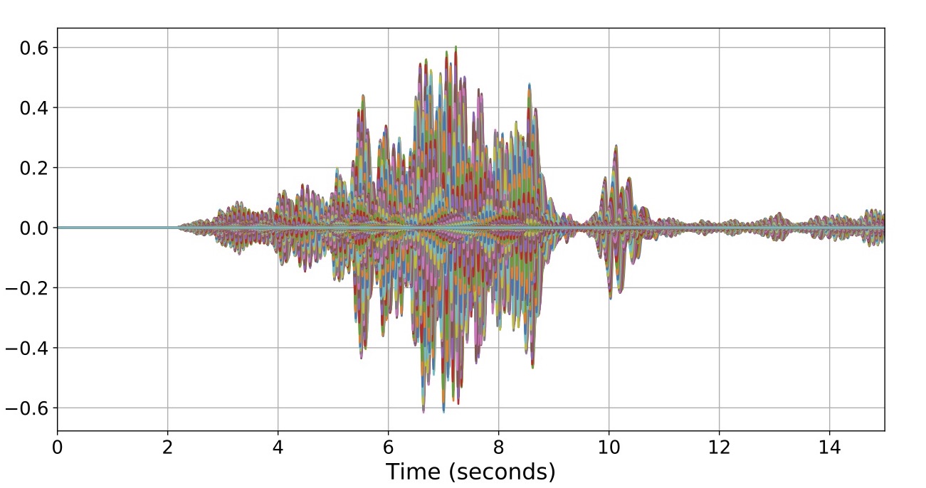
Narrow band filtered seismograms.
Animation 2: Normal Modes
The first 8 gravest (lowest frequency) spheroidal modes are extracted from 48 hour seismograms (Fig. 2). This animation shows the shapes of these modes in color and the superposition of the modes in white, starting from the lowest frequency and incrementally adding higher modes. Each mode is mapped to a tone that we can hear, where the relative frequencies of the tones are preserved. By the end of the animation, you can begin to see surface waves propagating back and forth.
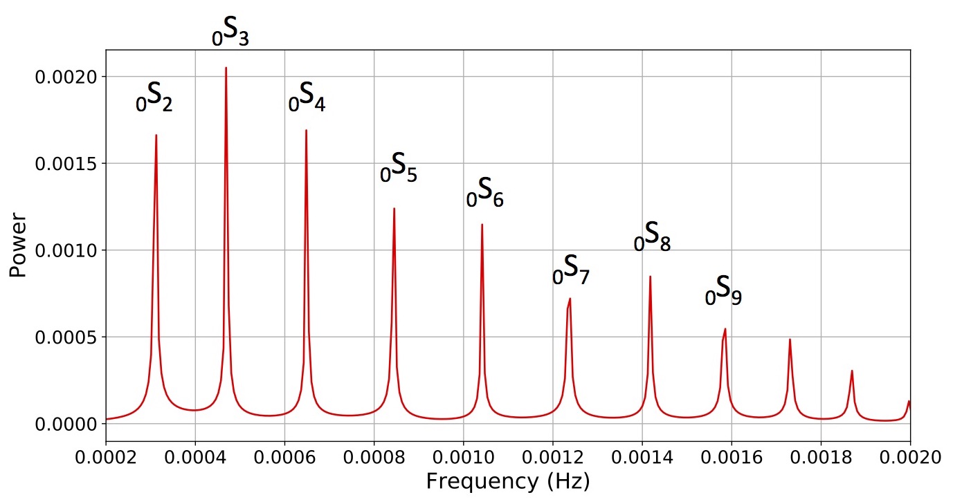
Discrete frequencies for the 8 gravest modes.
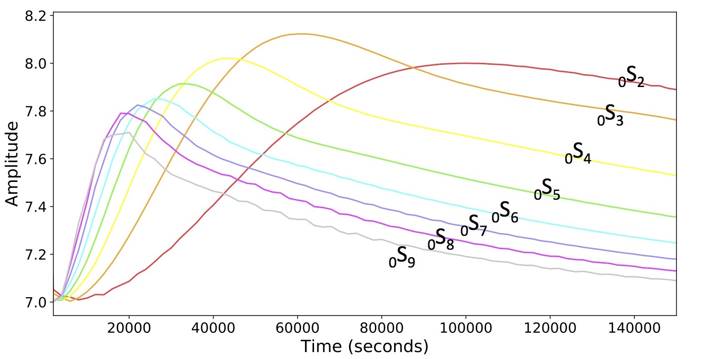
Animation 3: Attenuation
This animation is similar to Animation 2 except this time, all the modes are played at once. The tone of each mode is modulated in time by the amplitude envelopes in Fig. 3. Through time, the high frequencies die out due to anelastic attenuation and all that is left are the lowest frequency modes. In this video, you can actually hear this attenuation!